Simulation Output
This document describes the content and format of the output file produced by the simulate program.
The output consists of a FITS file containing several header/data units (HDUs).
You can inspect an output file’s contents from an interactive python session, e.g.:
import fitso
fits = fitsio.FITS('demo.fits')
print fits[0] # simulated survey image
print fits[1] # analysis results
fits.close()
You can reconstruct the analysis descwl.analysis.OverlapResults using the descwl.output.Reader class, e.g.:
import descwl
results = descwl.output.Reader('demo.fits').results
print results.survey.description()
You will need to ensure that the descwl package directory is in your $PYTHONPATH for this example to work. See the skeleton program for a more complete example of using analysis results from python.
Simulated Survey Image
The primary HDU contains the final simulated image using double precision floats. All sources are superimposed in this source and fluxes are given in units of detected electrons during the full exposure time.
All of the descwl.survey.Survey constructor args are saved as header keywords in the primary HDU, using only the last eight characters in upper case for the corresponding keys. In addition, the class attribute variables listed below are saved to the header.
| Key | Class | Attribute | Description |
|---|---|---|---|
| NSLICES | descwl.analysis.OverlapResults | num_slices | Number of slices for each per-object datacube |
| PSF_SIGM | descwl.survey.Survey | psf_sigma_m | PSF size |Q|**0.25 in arcsecs (unweighted Q) |
| PSF_SIGP | descwl.survey.Survey | psf_sigma_m | PSF size (0.5*trQ)**0.5 in arcsecs (unweighted Q) |
| PSF_HSM | descwl.survey.Survey | psf_size_hsm | PSF size |Q|**0.25 in arcsecs (weighted Q) |
To write a survey image with Poisson sky noise added to a new file, use e.g.:
import galsim,descwl
results = descwl.output.Reader('LSST_i.fits').results
results.add_noise(noise_seed=1)
galsim.fits.write(results.survey.image,'LSST_i_noise.fits')
Analysis Results
HDU[1] contains a binary table where each row represents one simulated source and the columns are described in the table below. Q refers to the second-moment tensor of the galaxy’s combined (bulge + disk + AGN) 50% isophote, including any cosmic shear but not the PSF. M refers to the second-moment tensor estimated using adaptive pixel moments and including the PSF. Note that the e1,e2 and hsm_e1,hsm_e2 parameters use different ellipticity conventions. HSM below refers to algorithms described in Hirata & Seljak (2003; MNRAS, 343, 459) and tested/characterized using real data in Mandelbaum et al. (2005; MNRAS, 361, 1287).
| Name | Type | Description |
|---|---|---|
| db_id | int64 | Unique identifier for this source in the LSST DM catalog database |
| grp_id | int64 | Group identifier (db_id of group member with largest snr_grp) |
| grp_size | int16 | Number of sources in this group (equal to 1 for isolated sources) |
| grp_rank | int16 | Rank position of this source in its group based on decreasing snr_iso |
| visible | int16 | Is this source’s centroid within (1) our outside (0) the simulated image bounds? |
| Stamp Bounding Box | ||
| xmin | int32 | Pixel offset of left edge of bounding box relative to left edge of survey image |
| xmax | int32 | Pixel offset of right edge of bounding box relative to left edge of survey image |
| ymin | int32 | Pixel offset of bottom edge of bounding box relative to bottom edge of survey image |
| ymax | int32 | Pixel offset of top edge of bounding box relative to bottom edge of survey image |
| Source Properties | ||
| f_disk | float32 | Fraction of total galaxy flux to due a Sersic n=1 disk component |
| f_bulge | float32 | Fraction of total galaxy flux to due a Sersic n=4 bulge component |
| dx | float32 | Source centroid in x relative to image center in arcseconds |
| dy | float32 | Source centroid in y relative to image center in arcseconds |
| z | float32 | Catalog source redshift |
| ab_mag | float32 | Catalog source AB magnitude in the simulated filter band |
| ri_color | float32 | Catalog source color calculated as (r-i) AB magnitude difference |
| flux | float32 | Total detected flux in electrons |
| sigma_m | float32 | Galaxy half-light radius in arcseconds calculated as |Q|**0.25 |
| sigma_p | float32 | Galaxy half-light radius in arcseconds calculated as (0.5*trQ)**0.5 |
| e1 | float32 | Real part (+) of galaxy ellipticity spinor (Q11-Q22)/(Q11+Q22+2|Q|**0.5) |
| e2 | float32 | Imaginary part (x) of galaxy ellipticity spinor (2*Q12)/(Q11+Q22+2|Q|**0.5) |
| a | float32 | Semi-major axis of 50% isophote ellipse in arcseconds, derived from Q |
| b | float32 | Semi-minor axis of 50% isophote ellipse in arcseconds, derived from Q |
| beta | float32 | Position angle of second-moment ellipse in radians, or zero when a = b |
| psf_sigm | float32 | PSF-convolved half-light radius in arcseconds calculated as |Q|**0.25 |
| Pixel-Level Properties | ||
| purity | float32 | Purity of this source in the range 0-1 (equals 1 when grp_size is 1) |
| snr_sky | float32 | S/N ratio calculated by ignoring any overlaps in the sky-dominated limit (a) |
| snr_iso | float32 | Same as snr_sky but including signal variance (b) |
| snr_grp | float32 | Same as snr_sky but including signal+overlap variance (c) |
| snr_isof | float32 | Same as snr_grp but including correlations with fit parameters for this source (d) |
| snr_grpf | float32 | Same as snr_grp but including correlations with fit parameters for all sources (e) |
| ds | float32 | Error on scale dilation factor (nominal s=1) marginalized over flux,x,y,g1,g2 (d) |
| dg1 | float32 | Error on shear + component (nominal g1=0) marginalized over flux,x,y,scale,g2 (d) |
| dg2 | float32 | Error on shear x component (nominal g2=0) marginalized over flux,x,y,scale,g1 (d) |
| ds_grp | float32 | Same as ds but also marginalizing over parameters of any overlapping sources (e) |
| dg1_grp | float32 | Same as dg1 but also marginalizing over parameters of any overlapping sources (e) |
| dg2_grp | float32 | Same as dg2 but also marginalizing over parameters of any overlapping sources (e) |
| HSM Analysis Results (ignoring overlaps) | ||
| hsm_sigm | float32 | Galaxy size |M|**0.25 in arcseconds from PSF-convolved adaptive second moments |
| hsm_e1 | float32 | Galaxy shape e1=(M11-M22)/(M11+M22) from PSF-convolved adaptive second moments |
| hsm_e2 | float32 | Galaxy shape e1=(2*M12)/(M11+M22) from PSF-convolved adaptive second moments |
| Systematics Fit Results | ||
| g1_fit | float32 | Best-fit value of g1 from simultaneous fit to noise-free image |
| g2_fit | float32 | Best-fit value of g2 from simultaneous fit to noise-free image |
The figure below illustrates the different Fisher-matrix error-estimation models (a-e) used to define the pixel-level properties and referred to in the table above. The green bands show the variance used in the Fisher-matrix denominator and the arrows indicate the parameters that are considered floating for calculating marginalized parameter errors. Vertical arrows denote flux parameters and horizontal arrows denote the size and shape parameters (dx,dy,ds,dg1,dg2).
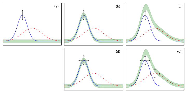
If any Fisher matrix is not invertible or yields non-positive variances, galaxies are iteratively dropped (in order of increasing snr_iso) until a valid covariance is obtained for the remaining galaxies. The corresponding values in the analysis results table will be zero for signal-to-noise ratios and infinite (numpy.inf) for errors on s,g1,g2.
You can load just the analysis results catalog from the output file using, e.g.:
import astropy.table
catalog = astropy.table.Table.read('demo.fits',hdu=1)
To scroll through the table in an interactive python session, use:
catalog.more()
To browse the catalog interactively (including seaching and sorting), use:
catalog.show_in_browser(jsviewer=True)
To plot a histogram of signal-to-noise ratios for all visible galaxies (assuming that matplotlib is configured):
plt.hist(catalog['snr'][catalog['visible']])
Rendered Galaxy Stamps
HDU[n+1] contains an image data cube for stamp n = 0,1,... Each data cube HDU has header keywords X_MIN and Y_MIN that give the pixel offset of the stamp’s lower-left corner from the lower-left corner of the full simulated survey image. Note that stamps may be partially outside of the survey image, but will always have some pixels above threshold within the image.
DS9 Usage
If you open an output file with the DS9 program you will normally only see the full simulated survey image in the primary HDU. You can also use the File > Open As > Multiple Extension Cube... to view the nominal rendered stamp for each visible galaxy (but not any partial derivative images).