Programs
All available programs are contained in the top-level directory where this package is installed. Programs are written in python and use the ‘.py’ file extension.
All programs are configured by passing command-line options. Pass the –help option to view documentation for these options, e.g.:
./simulate.py --help
Note that some program arguments normally contain characters that your shell may interpret specially but you can generally avoid this by quoting these arguments. For example, the square brackets [ ] and parentheses ( ) in the following command line are problematic and should be quoted as shown:
./display.py -i demo --crop --select-region '[-10.20,2.80,-30.40,-12.80]' --info '%(grp_size)d' --magnification 8
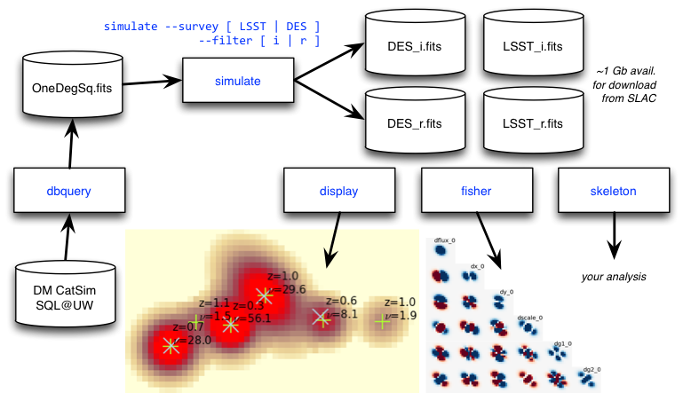
This document provides an introduction to each of the available programs. Examples of running the programs are documented elsewhere. The flowchart below shows the main processing steps and relationships between these programs.
simulate
The simulate program simulates and analyzes a weak-lensing survey by performing fast image rendering with galsim.
The program reads a catalog of astronomical sources and produces a set of output data products. Simulation outputs can be displayed with the display and fisher programs, or you can modify the skeleton program to perform your own analysis of the outputs.
By default, the program will simulate and analyze an area corresponding to 1 LSST chip (about 13 x 13 arcmin**2) assuming a full-depth LSST i-band exposure with nominal PSF, sky background, extinction, zero points, etc. To simulate a different nominal survey use, e.g.:
./simulate.py --survey LSST --filter r
./simulate.py --survey DES --filter i
Use the following command to see all the defaults associated with each survey configuration:
./simulate.py --survey-defaults
You can override any of these defaults on the command line, e.g.:
./simulate.py --survey CFHT --sky-brightness 20.7 --airmass 1.3 --atmospheric-psf-e1 0.01
You can also create new default survey configurations by editing the descwl.survey module.
The main simulation parameter is the pixel signal-to-noise threshold, min-snr:
./simulate.py --min-snr 0.1 ...
Sources are simulated over a footprint that includes exactly those pixels whose noise-free mean signal is above this threshold. Any source with at least one pixel meeting this criterion is considered ‘visible’ and others are discarded from the subsequent analysis and output. The threshold is in units of the full-depth mean sky noise level and the default value is 0.05.
For a full list of the available options, use:
./simulate.py --help
For details on the simulation output format, see this page.
display
The display program displays simulated images and analysis results stored in the FITS file generated by the simulate program.
Certain objects can be selected for highlighting and annotating. Use the –galaxy command-line arg to select a single galaxy using its unique database identifier (db_id in the Analysis Results). Similarly, use –group to select all galaxies in an overlapping group identified by its grp_id. The –galaxy and –group args can be repeated and combined and the resulting selection is the logical OR of each specification. More generally, objects can be selected using any expression of the variables in the Analysis Results with the –select option. For example, the following args select objects that are visible and pass a minimum signal-to-noise ratio cut:
./display.py --select 'visible' --select 'snr_iso > 10' ...
The –select arg can be repeated and the results will be combined with logical AND, followed by the logical OR of any –galaxy or –group args.
Displayed pixel values are clipped using an upper limits set at a fixed percentile of the histogram of non-zero pixel values for the selected objects, and a lower limit set a a fixed fraction of the mean sky noise level. Use the –clip-hi-percentile and –clip-lo-noise-fraction command-line args to change the defaults of 90% and 0.1, respectively. Clipped pixel values are rescaled from zero to one and displayed using the DS9 sqrt scale.
Scaled pixel values are displayed using two colormaps: one for selected objects and another for background objects. Use the –highlight and –colormap command-line args to change the defaults using any named matplotlib colormap.
Selected objects can be annotated using any information stored in the Analysis Results. Annotations are specified using python format strings where all catalog variables are available. For example, to display redshifts with 2 digits of precision, use:
./display.py --info '%(z).2f' ...
More complex formats with custom styling options are also possible, e.g.:
./display.py --info '$\\nu$ = %(snr_isof).1f,%(snr_grpf).1f' --info-size large --info-color red ...
The results of running an independent object detection pipeline can be superimposed in a displayed image. The match-catalog option specifies the detections to use in SExtractor compatible format. The matching algorithm is described here. Matches can also be annoted, e.g.:
./display.py --match-catalog SE.cat --match-info '%(FLUX_AUTO).1f'
For a full list of available options, use:
./display.py --help
fisher
The fisher program creates plots to illustrate galaxy parameter error estimation using Fisher matrices.
The program either calculates the Fisher matrix for a single galaxy (–galaxy) as if it were isolated, or else for an overlapping group of galaxies (–group). The displayed image consists of the lower-triangular part of a symmetric npar x npar matrix, where:
npar = (num_partials=6) * num_galaxies
By default, the program displays the Fisher-matrix images whose sums (over pixels) give the Fisher matrix element values. Alternatively, you can display the partial derivative images (–partials), Fisher matrix elements (–matrix), covariance matrix elements (–covariance) or correlation coefficients matrix (–correlation).
Use the –colormap option to select the color map. The vertical color scales are optimized independently for each partial-derivative or Fisher-matrix image, but are guaranteed to use ranges that are symmetric about zero (so diverging colormaps are usually the best choice). When Fisher or covariance matrix elements are being displayed, their relative values are somewhat arbitrary since they generally have different units. However, the dimensionless correlation coefficient matrix is always displayed using a scale range of [-1,+1].
skeleton
The skeleton program provides a simple demonstration of reading and analyzing simulation output that you can adapt to your own analysis. See the comments in the code for details.
dbquery
The dbquery program queries the official LSST simulation galaxy catalog and writes a text catalog file in the format expected by the simulate program. You do not normally need to run this program since suitable catalog files are already provided.